first level titleCurve Finance

Original compilation:JamesX，iZUMi Research

Overview

The design of the stablecoin has few concepts: lending-liquidating amm algorithm (LLAMMA), PegKeeper, Monetary Policy are the most important ones. But the main idea is in LLAMMA: replacing liquidations with a special-purpose AMM.

image description

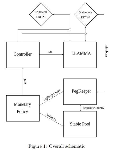
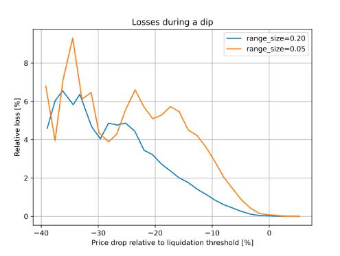
Figure 2 : Dependence of the loss on the price shift relative to the liquidation threshold. Time window for the observation is 3 days

text

In this design, if someone borrows against collateral, even at liquidation threshold, and the price of collateral dips and bounces - no significant loss happen. For example, according to simulations using historic data for ETH/USD since Sep 2017 , if one leaves the CDP unattended for 3 days and during this time the price drop of 10% below the liquidation threshold happened - only 1% of collateral gets lost.

secondary title

AMM for continuous liquidation/deliquidation (LLAMMA)

Continuous liquidation/AMM without liquidation (LLAMMA)

The core idea of the stablecoin design is Lending-Liquidating AMM Algorithm. The idea is that it converts between collateral (for example, ETH) and the stablecoin (let’s call it USD here). If the price of collateral is high - a user has deposits all in ETH, but as it goes lower, it converts to USD. This is very different from traditional AMM designs where one has USD on top and ETH on the bottom instead.

The core idea of ​​stablecoin design is the Lending-Liquidating AMM algorithm. The idea is that it converts between collateral (e.g. ETH) and a stablecoin (let’s call it USD here). If the price of the collateral is high - the user's deposit is all in ETH, but when the price is lower, it is converted to the USD stablecoin. This is very different from the traditional AMM design. The traditional AMM design is to place the USD stablecoin on the top (the upper half of the AMM curve) and ETH on the bottom (the lower half of the AMM curve).

The below description doesn’t serve as fully self-consistent rigorous proofs. A lot of that (especially the invariant) are obtained from dimensional considerations. More research might be required to have a full mathematical description, however the below is believed to be enough to implement in practice.

The following description does not serve as a fully self-consistent rigorous proof. Many things (especially invariants) are considered from various dimensions. To have a complete mathematical description, more research may be required, however the description below is considered sufficient to support implementation in smart contracts.

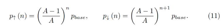
This is only possible with an external price oracle. In a nutshell, if one makes a typical AMM (for example with a bonding curve being a piece of hyperbola) and ramps its “center price” from (for example) down to up, the tokens will adiabatically convert from (for example) USD to ETH while proving liquidity in both ways on the way (Fig. 3 ). It is somewhat similar to avoided crossing (also called Landau-Zener transition) in quantum physics (though only as an idea: mathematical description of the process could be very different). The range where the liquidity is concentrated is called band here, at the constant po band has liquidity from pcd to pcu. We seek for pcd(po) and pcu(po) being functions of po only, functions being more steep than linear and, hence, growing faster than po(Fig. 4 ). In addition, let’s defifine prices p↓and p↑ being prices where p↓(po) = po, and p↑(po) = po, defining ends of bands in adiabatic limit (e.g. p = po).

This is only possible through price feeds from external oracles. In short, if one takes a typical AMM (for example, the bonding curve is a piece of hyperbola), and puts"center price"To go from (say) down to up, the token will "adiabatically" convert from (say) USD to ETH, while providing liquidity both ways in the process (Figure 3). This is somewhat analogous to "avoiding crossings" (also known as Landau-Zener transitions) in quantum physics (although just a concept: the mathematical description of the process can be very different).

image description

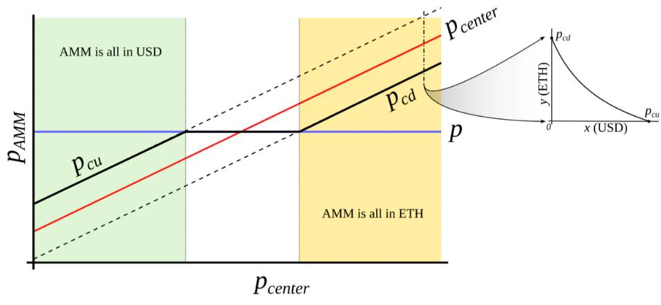Figure 3 : Behavior of an “AMM with an external price source”. External price pcenter determines a price around which liquidity is formed. AMM supports liquidity concentrated from prices pcd to pcu, pcd < pcenter < pcu. When current price p is out of range between pcd and pcu, AMM is either fully in stablecoin (when at pcu) or fully in collateral (when at pcd). When pcd ≤ p ≤ pcu, AMM price is equal to the current price p.

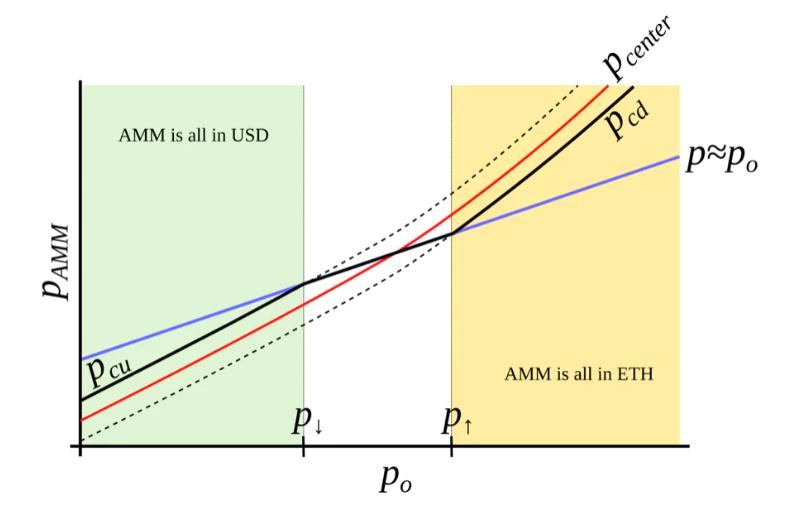Figure 4 : AMM which we search for. We seek to construct an AMM where pcd and pcu are such functions of po that when po grows, they grow even faster. In this case, this AMM will be all in ETH when ETH is expensive, and all in USD when ETH is cheap.

We start from a number of bands where, similarly to Uniswap 3 , hyperbolic shape of the bonding curve is preserved by adding virtual balances. Let say, the amount of USD is x, and the amount of ETH is y, therefore the “amplifified” constant-product invariant would be:

We start with some bands, similar to Uniswap 3, by adding "virtual balances", preserving the hyperbolic shape of the bonding curve. Let's say the amount of USD is x and the amount of ETH is y, so"Enhanced"Constant - Product invariant will be:

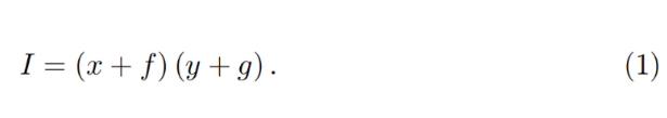
We also can denote x 0 ≡ x  +  f and y 0 ≡ y + g so that the invariant can be written as a familiar I =  x 0 y 0. However, f and g do not stay constant: they change with the external price oracle (and so does the invariant I, so it is only the invariant while the oracle price po is unchanged). At a given po, f and g are constant across the band. As mentioned before, we denote p↑ as the top price of the band and p↓as the bottom price of the band. We defifine A (a measure of concentration of liquidity) in such a way that:

We can also express x 0 ≡x+f and y 0 ≡y+g, so that the invariant can be written as the familiar I=x 0 y 0 . However, f and g are not constant: they change as the external oracle price changes (as does the invariant I, so it is only invariant when the oracle price po is constant). At a given po, f and g are constant across the band. As before, we denote p↑ as the top price of the band and p↓ as the bottom price of the band. Our definition of A (a measure of liquidity concentration) is as follows:

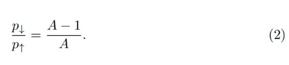
The property we are looking for is such that higher price po should lead to even higher price at the same balances, so that the current market price (which will, on average, follow po) is lower than that, and the band will trade towards being all in ETH (and the opposite is also true for the other direction). It is possible to find many ways to satisfy that but we need one:

The property we are looking for is this: a higher price po should lead to a higher price for the same balance, so the current market price (on average, will follow po) is below this price and the band will move towards All transactions in the direction of ETH (and the other direction as well). Many ways can be found to satisfy, but we need this one:

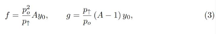
where y 0 is a p 0 -dependent measure of deposits in the current band, denominated in ETH, defifined in such a way that when current price p, p↑ and po are equal to each other, then y = y 0 and x = 0 (see the point at po = p↑ on Fig. 4 ). Then if we substitute y at that moment:

Among them, y 0 is an indicator related to p 0 to measure the current band deposit, and it is in ETH. Its definition is: when the current price p, p↑ and po are equal to each other, then y=y 0 , x= 0 (see The point of po=p↑ in Figure 4). So, if we replace y at that moment:

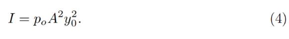
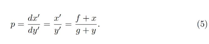
Price is equal to dx 0 /dy 0 which then for a constant-product invariant is:

price is equal to dx 0 /dy 0 , then for a constant product invariant, it is:

One can substitute situations where po = p↑ or po = p↓ with x = 0 or y = 0 correspndingly to verify that the above formulas are self-consistent.

We can use x= 0 or y= 0 to replace po=p↑ or po=p↓ to verify that the above formula is self-consistent.

Typically for a band, we know p↑ and, hence, p↓, po, constant A, and also x and y (current deposits in the band). To calculate everything, we need to find yo. It can be found by solving the quadratic equation for the invariant:

Usually for a band, we know p↑ and therefore p↓, po, the constant A, and also x and y (the current deposit in the band). To calculate the rest, we need to find yo. It can be found by solving the quadratic equation for the invariants:

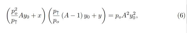
which turns into the quadratic equation against yo:

This becomes a quadratic equation for yo:

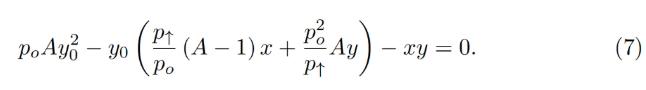
In the smart contract, we solve this quadratic equation in get_y 0 function.

In the smart contract, we solve this quadratic equation in the get_y 0 function.

While oracle price po stays constant, the AMM works in a normal way, e.g. sells ETH when going up / buys ETH when going down. By simply substituting x = 0 for the “current down” price pcd or y = 0 for the “current up” price pcu values into the equation of the invariant respectively, it is possible to show that AMM prices at the current value of po and the current value of p↑ are:

With the oracle price po remaining constant, the AMM works in the normal way, e.g. sell ETH when it goes up / buy ETH when it goes down. By simply replacing x= 0 with"current drop"The price of pcd or y= 0 is replaced by"current rise"Substituting the pcu value of the price of p into the invariant equation respectively, it can be shown that the AMM price under the current value of po and the current value of p↑ is:

Another practically important question is: if price changes up or down so slowly that the oracle price po is fully capable to follow it adiabatically, what amount y↑ of ETH (if the price goes up) or x↓ of USD (if the price goes down) will the band end up with, given current values x and y and that we start also at p = po. While it’s not an immediately trivial mathematical problem to solve, numeric computations showed a pretty simple answer:

Another important practical question: if the price changes so slowly that the oracle price po is perfectly able to follow it "adiabatically" (within a band), then given current values ​​x and y, and we also start from When p=po starts, how much y↑ of ETH (if the price goes up) or x↓ of USD (if the price goes down) will this band end up getting. While this is not an immediately solvable mathematical problem, numerical calculations reveal a fairly simple answer:

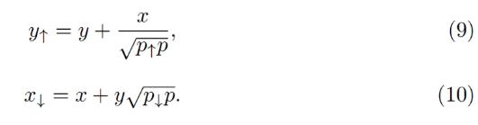
We will use these results when evaluating safety of the loan as well as the potential losses of the AMM.

We will use these results when evaluating the safety of lending and the potential loss of AMMs.

Now we have a description of one band. We split all the price space into bands which touch each other with prices p↓ and p↑ so that if we set a base price pbase and have a band number n:

Now we have a description of a band. We divide all the price space into bands whose prices p↓ and p↑ touch each other, so if we set a base price pbase with a band number n:

It is possible to prove that the solution of Eq. 7 and Eq. 5 for any band gives:

For any band, it can be shown that the solutions of Equation 7 and Equation 5 can be obtained:

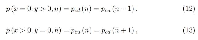
which shows that there are no gaps between the bands.

This shows that there are no gaps between the bands.

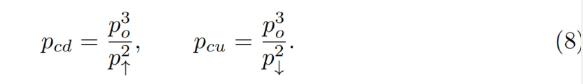
Trades occur while preserving the invariant from Eq. 1 , however the current price inside the AMM shifts when the price po: it goes up when po goes down and vice versa cubically, as can be seen from Eq. 8.

first level title

LLAMMA vs Stablecoin

Stablecoin is a CDP where one borrows stablecoin against a volatile collateral (cryptocurrency, for example, against ETH). The collateral is loaded into LLAMMA in such a price range (such bands) that if price of collateral goes down relatively slowly, the ETH gets converted into enough stablecoin to cover closing the CDP (which can happen via a self-liquidation, or via an external liquidation if the coverage is too close to dangerous limits, or not close at all while waiting for the price bounce).

Stablecoins are a type of CDP that people borrow against volatile collateral (a cryptocurrency such as ETH). Collateral is loaded into LLAMMA's price range (such a band), and if the price of the collateral falls relatively slowly, ETH is converted into enough stablecoins to cover closing the CDP (this can happen through self-liquidation, or through external liquidation, If the mortgage rate is too close to the dangerous limit, or not close at all, while waiting for the price to rebound).

When a user deposits collateral and borrows a stablecoin, the LLAMMA smart contract calculates the bands where to locate the collateral.  When the price of the collateral changes, it starts getting converted to the stablecoin. When the system is “underwater”, user already has enough USD to cover the loan. The amount of stablecoins which can be obtained can be calculated using a public get_x_down method. If it gives values too close to the liquidation thresholds - an external liquidator can be involved (typically shouldn’t happen within a few days or even weeks after the collateral price went down and sideways, or even will not happen ever if collateral price never goes up or goes back up relatively quickly). A health method returns a ratio of get_x_down to debt plus the value increase in collateral when the price is well above “liquidation”.

When a user deposits collateral and borrows a stablecoin, the LLAMMA smart contract calculates which band the collateral is in. When the price of the collateral changes, it starts being converted into a stablecoin. When the system is in"underwater", the user already has enough USD to pay the loan. The amount of stablecoins that can be obtained can be calculated through a public get_x_down method. If it gives a value that is too close to the liquidation threshold - external liquidators can get involved (which usually shouldn't happen in the days or even weeks after collateral prices fall and go sideways, even if collateral prices never rise or are relatively faster pick-up, it will never happen). when the price is much higher than"to liquidate", a healthy method returns the ratio of get_x_down to debt, plus the increase in value of the collateral.

When a stablecoin charges interest, this should be reflected in the AMM, too. This is done by adjusting all the grid of prices. So, when a stablecoin charges interest rate r, all the grid of prices in the AMM shifts upwards with the same rate r which is done via a base_price multiplier. So, the multiplier goes up over time as long as the charged rate is positive.

When a stablecoin charges interest, this should be reflected in the AMM. It must also be reflected. This is achieved by adjusting all grids for prices. So when a stablecoin charges an interest rate r, all prices in the AMM move upwards with the same interest rate r, and this is done via a base price multiplier. So, as long as the rate charged is positive, the multiplier will go up over time.

When we calculate get_x_down or get_y_up, we are first looking for the amounts of stablecoin and collateral x∗ and y∗ if current price moves to the current price po. Then we look at how much stablecoin or collateral we get if po adiabatically changes to either the lowest price of the lowest band, or the highest price of the highest band respectively. This way, we can get a measure of how much stablecoin we will which is not dependent on the current instantaneous price, which is important for sandwich attack resistance.

When we calculate get_x_down or get_y_up, the first thing we look for is the amount of stablecoin and collateral x∗ and y∗ if the current price moves to the current price po. Then we see, if po changes adiabatically to the lowest price in the lowest range, or the highest price in the highest range, how many stablecoins or collateral we get respectively. In this way, we can get a measure of how much stablecoin we will get, which does not depend on the current instantaneous price, which is important for the resistance of mezzanine attacks. **
**

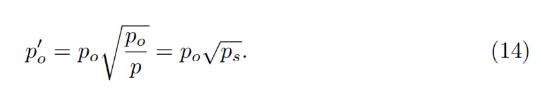
It is important to point out that the LLAMMA uses po defined as ETH/USD price as a price source, and our stablecoin could be traded under the peg (ps < 1 ) or over peg (ps > 1 ). If ps < 1 , then price in the LLAMMA is p > po.

It should be pointed out that LLAMMA uses po defined as the price of ETH/USD as a price source, and our stablecoin can be traded below the peg (ps<1) or above the peg (ps>1). if ps<1 , then the price in LLAMMA is p>po.

In adiabatic approximation, p = po/ps, and all the collateral<>stablecoin conversion would happen at a higher oracle price / as if oracle price was lower and equal to:

In the adiabatic approximation, p=po/ps, all collateral<>Stablecoin conversion will happen at higher oracle price / as if oracle price is lower and equal to:

At this price, the amount of stablecoins obtained at conversion is higher by factor of 1/ps (if ps < 1 ) .

At this price, the number of stable coins obtained when converting is higher by a factor of 1/ps (if ps<1 ）。

It is less desirable to have ps > 1 for prolonged times, and for that we will use the stabilizer (see next)

Automatic Stabilizers and Monetary Policy

Automatic Stabilizer and Monetary Policy

Automatic Stabilizers and Monetary Policy

When ps > 1 (for example, because of the increased demand for stablecoin), there is peg-keeping reserve formed by an asymmetric deposit into a stableswap Curve pool between the stablecoin and a redeemable reference coin or LP token. Once ps > 1 , the PegKeeper contract is allowed to mint uncollateralized stablecoin and (only!) deposit it to the stableswap pool single-sided in such a way that the final price after this is still no less than 1. When ps < 1 , the PegKeeper is allowed to withdraw (asymmetrically) and burn the stablecoin.

When ps > 1 (e.g. due to increased demand for stablecoins), there will be pegged reserves formed by asymmetric deposits between stablecoins and redeemable reference coins or LP tokens to the stableswap Curve pool . Once ps>1, the PegKeeper contract is allowed to mint unsecured stablecoins and only deposit them in the stableswap pool on one side, and the final price after doing so is still not lower than 1. when ps< 1, PegKeeper is allowed to withdraw (asymmetrically) and burn stablecoins.

These actions cause price ps to quickly depreciate when it’s higher than 1 and appreciate if lower than 1 because asymmetric deposits and withdrawals change the price. Even though the mint is uncollateralized, the stablecoin appears to be implicitly collateralized by liquidity in the stablecoin pool. The whole mint/burn cycle appears, at the end, to be profitable while providing stability.

These actions cause the price ps to rapidly depreciate above 1 and appreciate below 1 as asymmetric deposits and withdrawals change the price. Even though this portion of the "minting" is uncollateralized, the stablecoin appears to be backed by an implicit collateralization of liquidity in the stablecoin pool. The whole minting/burning cycle seems profitable in the end while providing stability.

Let’s denote the amount of stablecoin minted to the stabilizer (debt) as dst and the function which calculates necessary amount of redeemable USD to buy the stablecoin in a stableswap AMM get_dx as fdx(). Then, in order to keep reserves not very large, we use the “slow” mechanism of stabilization via varying the borrow r:

Let's denote the amount of stablecoins minted to the stablecoin (debt) as dst and the function to calculate the amount of redeemable USD needed to buy the stablecoin in the stableswap AMM get_dx as fdx(). Then, to keep the "reserve" from being very large, we use"slow"stabilization mechanism.

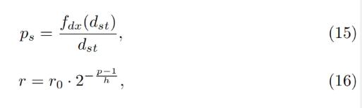
where h is the change in ps at which the rate r changes by factor of 2 (higher ps leads to lower r). The amount of stabilizer debt dst will equilibrate at different value depending on the rate at ps = 1 r 0. Therefore, we can (instead of setting manually) be reducing r 0 while dst/supply is larger than some target number (for example, 5%) (thereby incentivizing borrowers to borrow-and-dump the stablecoin, decreasing its price and forcing the system to burn the dst) or increasing if it’s lower (thereby incentivizing borrowers to return loans and pushing ps up, forcing the system to increase the debt dst and the stabilizer deposits).

first level title

Conclusion / summary

The presented mechanisms can, hopefully, solve the riskiness of liquidations for stablecoin-making and borrowing purposes. In addition, stabilizer and automatic monetary policy mechanisms can help with peg-keeping without the need of keeping overly big PSMs.

It is hoped that the proposed mechanism will address the risky nature of liquidations for stablecoin minting and lending purposes. In addition, stabilizers and automatic monetary policy mechanisms can help maintain price anchors without the need to maintain excessive PSM (Peg Stability Module anchor stability module).